python+matplotlib演示电偶极子实例代码
发布于 2018-02-15 22:28:03 | 174 次阅读 | 评论: 0 | 来源: 网友投递
这里有新鲜出炉的Python3 官方中文指南,程序狗速度看过来!
Python编程语言
Python 是一种面向对象、解释型计算机程序设计语言,由Guido van Rossum于1989年底发明,第一个公开发行版发行于1991年。Python语法简洁而清晰,具有丰富和强大的类库。它常被昵称为胶水语言,它能够把用其他语言制作的各种模块(尤其是C/C++)很轻松地联结在一起。
这篇文章主要介绍了python+matplotlib演示电偶极子实例代码,具有一定借鉴价值,需要的朋友可以参考下
使用matplotlib.tri.CubicTriInterpolator.演示变化率计算:
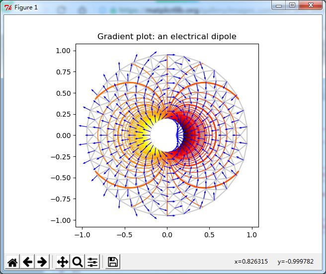
完整实例:
from matplotlib.tri import (
  Triangulation, UniformTriRefiner, CubicTriInterpolator)
import matplotlib.pyplot as plt
import matplotlib.cm as cm
import numpy as np


#-----------------------------------------------------------------------------
# Electrical potential of a dipole
#-----------------------------------------------------------------------------
def dipole_potential(x, y):
  """ The electric dipole potential V """
  r_sq = x**2 + y**2
  theta = np.arctan2(y, x)
  z = np.cos(theta)/r_sq
  return (np.max(z) - z) / (np.max(z) - np.min(z))


#-----------------------------------------------------------------------------
# Creating a Triangulation
#-----------------------------------------------------------------------------
# First create the x and y coordinates of the points.
n_angles = 30
n_radii = 10
min_radius = 0.2
radii = np.linspace(min_radius, 0.95, n_radii)

angles = np.linspace(0, 2 * np.pi, n_angles, endpoint=False)
angles = np.repeat(angles[..., np.newaxis], n_radii, axis=1)
angles[:, 1::2] += np.pi / n_angles

x = (radii*np.cos(angles)).flatten()
y = (radii*np.sin(angles)).flatten()
V = dipole_potential(x, y)

# Create the Triangulation; no triangles specified so Delaunay triangulation
# created.
triang = Triangulation(x, y)

# Mask off unwanted triangles.
triang.set_mask(np.hypot(x[triang.triangles].mean(axis=1),
             y[triang.triangles].mean(axis=1))
        < min_radius)

#-----------------------------------------------------------------------------
# Refine data - interpolates the electrical potential V
#-----------------------------------------------------------------------------
refiner = UniformTriRefiner(triang)
tri_refi, z_test_refi = refiner.refine_field(V, subdiv=3)

#-----------------------------------------------------------------------------
# Computes the electrical field (Ex, Ey) as gradient of electrical potential
#-----------------------------------------------------------------------------
tci = CubicTriInterpolator(triang, -V)
# Gradient requested here at the mesh nodes but could be anywhere else:
(Ex, Ey) = tci.gradient(triang.x, triang.y)
E_norm = np.sqrt(Ex**2 + Ey**2)

#-----------------------------------------------------------------------------
# Plot the triangulation, the potential iso-contours and the vector field
#-----------------------------------------------------------------------------
fig, ax = plt.subplots()
ax.set_aspect('equal')
# Enforce the margins, and enlarge them to give room for the vectors.
ax.use_sticky_edges = False
ax.margins(0.07)

ax.triplot(triang, color='0.8')

levels = np.arange(0., 1., 0.01)
cmap = cm.get_cmap(name='hot', lut=None)
ax.tricontour(tri_refi, z_test_refi, levels=levels, cmap=cmap,
       linewidths=[2.0, 1.0, 1.0, 1.0])
# Plots direction of the electrical vector field
ax.quiver(triang.x, triang.y, Ex/E_norm, Ey/E_norm,
     units='xy', scale=10., zorder=3, color='blue',
     width=0.007, headwidth=3., headlength=4.)

ax.set_title('Gradient plot: an electrical dipole')
plt.show()
总结
以上就是本文关于python+matplotlib演示电偶极子实例代码的全部内容,希望对大家有所帮助。感兴趣的朋友可以继续参阅本站其他相关专题,如有不足之处,欢迎留言指出。感谢朋友们对本站的支持!
您可能感兴趣的文章:
推荐阅读
最新资讯